Kinect Monte Carlo Simulations Using LAMMPS

Requirements

• You will need to install VOTCA using the instructions described here

• Once the installation is completed you need to activate the VOTCA enviroment by running the VOTCARC.bash script that has been installed at the bin subfolder for the path that you have provided for the installation step above

Setting the environment

We will use matplotlib, seaborn and pandas libraries for plotting. You can install it using pip like

!pip install seaborn --user

Requirement already satisfied: seaborn in /usr/lib/python3.13/site-packages (0.13.2)
Requirement already satisfied: numpy!=1.24.0,>=1.20 in /usr/lib64/python3.13/site-packages (from seaborn) (2.2.5)
Requirement already satisfied: pandas>=1.2 in /usr/lib64/python3.13/site-packages (from seaborn) (2.2.3)
Requirement already satisfied: matplotlib!=3.6.1,>=3.4 in /usr/lib64/python3.13/site-packages (from seaborn) (3.10.0)
Requirement already satisfied: contourpy>=1.0.1 in /usr/lib64/python3.13/site-packages (from matplotlib!=3.6.1,>=3.4->seaborn) (1.3.2)
Requirement already satisfied: cycler>=0.10 in /usr/lib/python3.13/site-packages (from matplotlib!=3.6.1,>=3.4->seaborn) (0.11.0)
Requirement already satisfied: fonttools>=4.22.0 in /usr/lib64/python3.13/site-packages (from matplotlib!=3.6.1,>=3.4->seaborn) (4.56.0)
Requirement already satisfied: kiwisolver>=1.3.1 in /usr/lib64/python3.13/site-packages (from matplotlib!=3.6.1,>=3.4->seaborn) (1.4.8)
Requirement already satisfied: packaging>=20.0 in /usr/lib/python3.13/site-packages (from matplotlib!=3.6.1,>=3.4->seaborn) (24.2)
Requirement already satisfied: pillow>=8 in /usr/lib64/python3.13/site-packages (from matplotlib!=3.6.1,>=3.4->seaborn) (11.1.0)
Requirement already satisfied: pyparsing>=2.3.1 in /usr/lib/python3.13/site-packages (from matplotlib!=3.6.1,>=3.4->seaborn) (3.1.2)
Requirement already satisfied: python-dateutil>=2.7 in /usr/lib/python3.13/site-packages (from matplotlib!=3.6.1,>=3.4->seaborn) (2.8.2)
Requirement already satisfied: pytz>=2020.1 in /usr/lib/python3.13/site-packages (from pandas>=1.2->seaborn) (2025.2)
Requirement already satisfied: six>=1.5 in /usr/lib/python3.13/site-packages (from python-dateutil>=2.7->matplotlib!=3.6.1,>=3.4->seaborn) (1.17.0)

Notes

• The ${VOTCASHARE} environmental variable is set to the path that you provided during the VOTCA installation, by the default is set to /usr/local/votca.

• In Jupyter the ! symbol means: run the following command as a standard unix command

• In Jupyter the command %env set an environmental variable

Site energies and pair energy differences

We will compute the histrogram using resolution_sites of 0.03 eV. See eanalyze options and defaults for more information.

!xtp_run -e eanalyze -c resolution_sites=0.03 -f state.hdf5

==================================================
========   VOTCA (http://www.votca.org)   ========
==================================================

please read and cite: https://doi.org/10.21105/joss.06864
and submit bugs to https://github.com/votca/votca/issues

xtp_run, version 2025-dev gitid: 7b6d1e5 (compiled May  2 2025, 05:53:28)

Initializing calculator
... eanalyze
1 frames in statefile, Ids are: 10000
Starting at frame 10000
Evaluating frame 10000
Import MD Topology (i.e. frame 10000) from state.hdf5
....
... eanalyze
 Using 1 threads
... ... Short-listed 1000 segments (pattern='*')
... ... ... NOTE Statistics of site energies and spatial correlations thereof are based on the short-listed segments only.
... ... ...      Statistics of site-energy differences operate on the full list.
... ... excited state e
... ... excited state h
... ... excited state s
... ... excited state t
Changes have not been written to state file.

In the current work directoy you can see the resulting files,

!ls eanalyze*

eanalyze.pairhist_e.out  eanalyze.pairlist_s.out  eanalyze.sitehist_e.out
eanalyze.pairhist_h.out  eanalyze.pairlist_t.out  eanalyze.sitehist_h.out
eanalyze.pairhist_s.out  eanalyze.sitecorr_e.out  eanalyze.sitehist_s.out
eanalyze.pairhist_t.out  eanalyze.sitecorr_h.out  eanalyze.sitehist_t.out
eanalyze.pairlist_e.out  eanalyze.sitecorr_s.out
eanalyze.pairlist_h.out  eanalyze.sitecorr_t.out

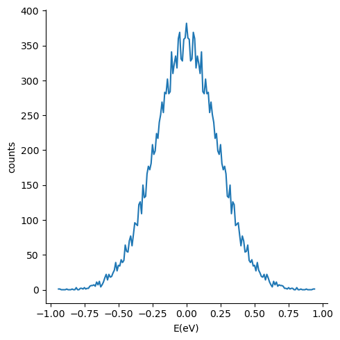
Plotting the energies

We will the previously installed pandas and seaborn library to plot the electron histrogram computed in the previous step,

import pandas as pd
import matplotlib.pyplot as plt
import seaborn as sns
columns = ["E(eV)", "counts"]
df = pd.read_table("eanalyze.pairhist_e.out", comment="#", sep='\s+',names=columns, skiprows=2)
sns.relplot(x="E(eV)", y="counts", ci=None, kind="line", data=df)
plt.plot()

<>:5: SyntaxWarning: invalid escape sequence '\s'
<>:5: SyntaxWarning: invalid escape sequence '\s'
/tmp/ipykernel_11559/2362228021.py:5: SyntaxWarning: invalid escape sequence '\s'
  df = pd.read_table("eanalyze.pairhist_e.out", comment="#", sep='\s+',names=columns, skiprows=2)
/usr/lib/python3.13/site-packages/seaborn/axisgrid.py:854: FutureWarning:

The `ci` parameter is deprecated. Use `errorbar=None` for the same effect.

  func(*plot_args, **plot_kwargs)

[]

Couplings histrogram

In this step we will analyze the electron/hole couplings, using the ianalyze calculator using the resolution_logJ2 parameter of 0.1 units. See the ianalyze options and defaults for more information about the calculator.

!xtp_run -e ianalyze -c resolution_logJ2=0.1 states=e,h -f state.hdf5

==================================================
========   VOTCA (http://www.votca.org)   ========
==================================================

please read and cite: https://doi.org/10.21105/joss.06864
and submit bugs to https://github.com/votca/votca/issues

xtp_run, version 2025-dev gitid: 7b6d1e5 (compiled May  2 2025, 05:53:28)

Initializing calculator
... ianalyze
1 frames in statefile, Ids are: 10000
Starting at frame 10000
Evaluating frame 10000
Import MD Topology (i.e. frame 10000) from state.hdf5
....
... ianalyze
 Using 1 threads
Calculating for state e now.
Calculating for state h now.
Changes have not been written to state file.

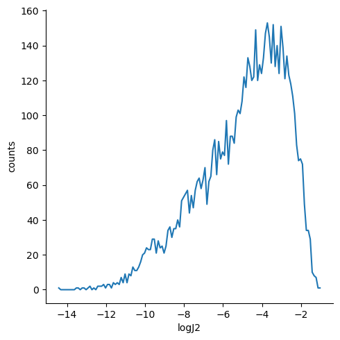
Plotting the coupling histogram

We can now plot the logarithm of the squared coupling for the hole,

columns = ["logJ2", "counts"]
df = pd.read_table("ianalyze.ihist_h.out", comment="#", sep='\s+',names=columns, skiprows=2)
sns.relplot(x="logJ2", y="counts", ci=None, kind="line", data=df)
plt.plot()

<>:2: SyntaxWarning: invalid escape sequence '\s'
<>:2: SyntaxWarning: invalid escape sequence '\s'
/tmp/ipykernel_11559/886975016.py:2: SyntaxWarning: invalid escape sequence '\s'
  df = pd.read_table("ianalyze.ihist_h.out", comment="#", sep='\s+',names=columns, skiprows=2)
/usr/lib/python3.13/site-packages/seaborn/axisgrid.py:854: FutureWarning:

The `ci` parameter is deprecated. Use `errorbar=None` for the same effect.

  func(*plot_args, **plot_kwargs)

[]

KMC simulations of multiple holes or electrons in periodic boundary conditions

Finally, lets do a 1000 seconds KMC simulation for the electron, with a 10 seconds window between output and a field of 10 V/m along the x-axis,

!xtp_run -e kmcmultiple -c runtime=1000 outputtime=10 field=10,0,0 carriertype=electron -f state.hdf5

==================================================
========   VOTCA (http://www.votca.org)   ========
==================================================

please read and cite: https://doi.org/10.21105/joss.06864
and submit bugs to https://github.com/votca/votca/issues

xtp_run, version 2025-dev gitid: 7b6d1e5 (compiled May  2 2025, 05:53:28)

Initializing calculator
... kmcmultiple
1 frames in statefile, Ids are: 10000
Starting at frame 10000
Evaluating frame 10000
Import MD Topology (i.e. frame 10000) from state.hdf5
....
... kmcmultiple
 Using 1 threads
 ...
-----------------------------------
      KMC FOR MULTIPLE CHARGES
-----------------------------------

 ...
Calculating initial rates.
 ... Rate engine initialized:
 Ratetype:marcus
 Temperature T[k] = 300
 Electric field[V/nm](x,y,z) =1e-08 0 0 ||F|| 1e-08

 ...
 ...     carriertype: electron
 ...     Rates for 1000 sites are computed.
 ...
Rates are written to rates.dat
 ... Nblist has 10151 pairs. Nodes contain 20302 jump events
with avg=20.302 std=2.07913 max=28 min=14 jumps per site
Minimum jumpdistance =0.366063 nm Maximum distance =1.10167 nm

 ... spatial carrier density: 0.00729374 nm^-3
 ...
Algorithm: VSSM for Multiple Charges
 ... number of carriers: 1
 ... number of nodes: 1000
 ... stop condition: 1000 steps.
 ... output frequency: every 10 steps.
 ... (If you specify runtimes larger than 100 kmcmultiple assumes that you are specifying the number of steps for both runtime and outputtime.)
 ... Writing trajectory to trajectory.csv.
 ... looking for injectable nodes...
 ... starting position for charge 0: segment 697
 ...
Occupations are written to occupation.dat
 ...
finished KMC simulation after 1000 steps.
simulated time 5.92255e-09 seconds.

 ...     carrier 1: 1.205058e+08 5.671523e+07 1.959596e+07
 ...   Overall average velocity (nm/s): 1.205058e+08 5.671523e+07 1.959596e+07
 ...
Distances travelled (nm):
 ...     carrier 1: 7.137019e-01 3.358990e-01 1.160581e-01
 ...
Mobilities (nm^2/Vs):
 ...     carrier 1: mu=1.205058e+16
 ...   Overall average mobility in field direction <mu>=1.205058e+16 nm^2/Vs
 ...
Eigenvalues:

 ... Eigenvalue: 2.670560e-09
 ... Eigenvector: 1.317081e-01   6.198754e-02   -9.893485e-01

 ... Eigenvalue: 2.670560e-09
 ... Eigenvector: 4.258378e-01   -9.047995e-01   0.000000e+00

 ... Eigenvalue: 5.366503e+07
 ... Eigenvector: -8.951621e-01   -4.213020e-01   -1.455661e-01
Changes have not been written to state file.

You can find both the occupation data and the rates for the electron at 300 K, on files occupation.dat and rates.dat, respectively.