DFT + GWBSE Energy Calculation Using CH4
Introduction
This tutorial explains how to perform calculation to predict electronic excitation using the GWBSE method. See the GW Compendium: A Practical Guide to Theoretical Photoemission Spectroscopy, for an excellent introduction to the method.
Requirements
You will need to install VOTCA using the instructions described here
Once the installation is completed you need to activate the VOTCA enviroment by running the
VOTCARC.bashscript that has been installed at the bin subfolder for the path that you have provided for the installation step above
Interacting with the XTP command line interface
To run a DFT-GWBSE calculation we will use the xtp_tools calculator. Run the following command to view the help message of xtp_tools:
[1]:
!xtp_tools --help
==================================================
========   VOTCA (http://www.votca.org)   ========
==================================================

please read and cite: https://doi.org/10.21105/joss.06864
and submit bugs to https://github.com/votca/votca/issues

xtp_tools, version 2026-dev gitid: 534a492 (compiled Jul 28 2026, 12:14:41)

Runs excitation/charge transport tools


Allowed options:
  -h [ --help ]                 display this help and exit
  --verbose                     be loud and noisy
  --verbose1                    be very loud and noisy
  -v [ --verbose2 ]             be extremly loud and noisy
  -o [ --options ] arg          Tool user options.
  -t [ --nthreads ] arg (=1)    number of threads to create
  -e [ --execute ] arg        Name of Tool to run
  -l [ --list ]               Lists all available Tools
  -d [ --description ] arg    Short description of a Tools
  -c [ --cmdoptions ] arg     Modify options via command line by e.g. '-c
                              xmltag.subtag=value'. Use whitespace to separate
                              multiple options
  -p [ --printoptions ] arg   Prints xml options of a Tool
Note
In Jupyter the
!symbol means: run the following command as a standard unix commandIn Jupyter the command
%envset an environmental variable
Running a calculation with the default options
To run a DFT-GWBSE calculation we just need to provide the path to the file in XYZ with the molecular coordinates. Check the dftgwbse defaults for further information.
[2]:
!xtp_tools -c job_name=methane -t 2 -e dftgwbse > dftgwbse.log
The previous command will run the DFT-GWBSE calculation using the aforementioned defaults and the results are store in the Current Work Directory in a file named methane_summary.xml. The -c option is important and we will come back to it later. It allows changing options form the command line.
Running a calculation using your own input file
Let create a folder to store the input options for XTP and use the -p option to print an option file, specified by -o, with all the options so we can modify it afterwards
[3]:
!mkdir -p OPTIONFILES
!xtp_tools -p dftgwbse -o OPTIONFILES/dftgwbse.xml
Writing options for calculator dftgwbse to OPTIONFILES/dftgwbse.xml
Done - stopping here
You should have a XML file with the DFTWGSE options that looks like
[4]:
!head -n 10 OPTIONFILES/dftgwbse.xml
<options>
<dftgwbse help="Compute electronic excitations using GW-BSE">
        <job_name default="system" help="Input file name without extension, also used for intermediate files">system</job_name>
        <dftpackage help="options for dftpackages">
                <name choices="xtp,orca" default="xtp" help="Name of the DFT package">xtp</name>
                <charge choices="int" default="0" help="Molecular charge">0</charge>
                <spin choices="int+" default="1" help="Molecular multiplicity">1</spin>
                <basisset default="def2-tzvp" help="Basis set for MOs">def2-tzvp</basisset>
                <auxbasisset default="OPTIONAL" help="Auxiliary basis set for RI"/>
                <externalfield default="OPTIONAL" help="Field given in x y z components" unit="Hartree/bohr"/>
Some options are labelled as OPTIONAL, either fill them in or delete them if you do not want that functionality
We created a small options file
[5]:
!cat dftgwbse2.xml
<options>
    <dftgwbse>
        <job_name>methane</job_name>
        <dftpackage>
            <basisset>ubecppol</basisset>
            <auxbasisset>aux-ubecppol</auxbasisset>
        </dftpackage>
    </dftgwbse>
</options>
[6]:
!xtp_tools -o dftgwbse2.xml -t 2 -e dftgwbse > dftgwbse2.log
XTP will automatically compare the default values with the user-provided and overwrites the defaults with the user input. Also, If I given property does not have a default value you can provide one using the XML file described above.
Partial Charges
We can compute now the partial charges using the CHELPG method by default. For more information see the partialcharges documentation. Once again, we only need to provide the name of the system to compute, which in our case is methane.
[7]:
!xtp_tools -c job_name=methane -e partialcharges
==================================================
========   VOTCA (http://www.votca.org)   ========
==================================================

please read and cite: https://doi.org/10.21105/joss.06864
and submit bugs to https://github.com/votca/votca/issues

xtp_tools, version 2026-dev gitid: 534a492 (compiled Jul 28 2026, 12:14:41)

Initializing tool
... partialcharges Evaluating tool
... partialcharges  Using 1 threads
... ...  Loading QM data from methane.orb
... ... ===== Running on 1 threads =====
... ... 2026-7-28 12:36:1 Calculated Densities at Numerical Grid, Number of electrons is -2.3744e-08
... ... 2026-7-28 12:36:1 Calculating ESP at CHELPG grid points
... ... 2026-7-28 12:36:3 Netcharge constrained to 0
... ...  Sum of fitted charges: 2.42133e-14
... ...  RMSE of fit:  0.0022159
... ...  RRMSE of fit: 0.107182
... ... El Dipole from fitted charges [e*bohr]:
                 dx = +0.7278 dy = -0.4713 dz = +0.4706 |d|^2 = +0.9733
... ... El Dipole from exact qm density [e*bohr]:
                 dx = +0.7620 dy = -0.4941 dz = +0.4932 |d|^2 = +1.0681
... ... Written charges to methane.mps
Spectrum Calculation
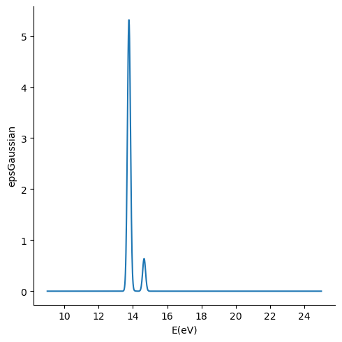
Finally, lets compute a convolution of the singlet spectrum using a gaussian function. For doing so, we will modify the default values for the spectrum calculator to compute the spectrum between 9 and 25 eV, using 1000 points in that energy range. We will use the -c option to modify the options accordingly. Instead we could have printed out an options file using the xtp_tools -p spectrum command and then modify the entries accordingly and
then read them in using the -o option.
[8]:
!xtp_tools -c job_name=methane lower=9 upper=25 points=1000 -e spectrum
==================================================
========   VOTCA (http://www.votca.org)   ========
==================================================

please read and cite: https://doi.org/10.21105/joss.06864
and submit bugs to https://github.com/votca/votca/issues

xtp_tools, version 2026-dev gitid: 534a492 (compiled Jul 28 2026, 12:14:41)

Initializing tool
... spectrum Evaluating tool
... spectrum  Using 1 threads
... ... Calculating absorption spectrum plot methane.orb
... ...  Loading QM data from methane.orb
... ...  Considering 10 excitation with max energy 14.6581 eV / min wave length 84.7406 nm
... ...  Spectrum in energy range from  9 to 25 eV and with broadening of FWHM 0.2 eV written to file  methane_spectrum.dat
The results are stored in the methane_spectrum.dat file.
(Optional) Plot the spectrum
We will use matplotlib, seaborn and pandas libraries to plot the spectrum. You can install it using pip like
[9]:
!pip install seaborn --user
Requirement already satisfied: seaborn in /usr/lib/python3.14/site-packages (0.13.2)
Requirement already satisfied: numpy!=1.24.0,>=1.20 in /usr/lib64/python3.14/site-packages (from seaborn) (2.4.6)
Requirement already satisfied: pandas>=1.2 in /usr/lib64/python3.14/site-packages (from seaborn) (2.3.3)
Requirement already satisfied: matplotlib!=3.6.1,>=3.4 in /usr/lib64/python3.14/site-packages (from seaborn) (3.10.8)
Requirement already satisfied: contourpy>=1.0.1 in /usr/lib64/python3.14/site-packages (from matplotlib!=3.6.1,>=3.4->seaborn) (1.3.3)
Requirement already satisfied: cycler>=0.10 in /usr/lib/python3.14/site-packages (from matplotlib!=3.6.1,>=3.4->seaborn) (0.11.0)
Requirement already satisfied: fonttools>=4.22.0 in /usr/lib64/python3.14/site-packages (from matplotlib!=3.6.1,>=3.4->seaborn) (4.62.1)
Requirement already satisfied: kiwisolver>=1.3.1 in /usr/lib64/python3.14/site-packages (from matplotlib!=3.6.1,>=3.4->seaborn) (1.5.0)
Requirement already satisfied: packaging>=20.0 in /usr/lib/python3.14/site-packages (from matplotlib!=3.6.1,>=3.4->seaborn) (25.0)
Requirement already satisfied: pillow>=8 in /usr/lib64/python3.14/site-packages (from matplotlib!=3.6.1,>=3.4->seaborn) (12.2.0)
Requirement already satisfied: pyparsing>=3 in /usr/lib/python3.14/site-packages (from matplotlib!=3.6.1,>=3.4->seaborn) (3.1.2)
Requirement already satisfied: python-dateutil>=2.7 in /usr/lib/python3.14/site-packages (from matplotlib!=3.6.1,>=3.4->seaborn) (2.9.0.post0)
Requirement already satisfied: pytz>=2020.1 in /usr/lib/python3.14/site-packages (from pandas>=1.2->seaborn) (2026.1)
Requirement already satisfied: six>=1.5 in /usr/lib/python3.14/site-packages (from python-dateutil>=2.7->matplotlib!=3.6.1,>=3.4->seaborn) (1.17.0)
[10]:
import pandas as pd
import matplotlib.pyplot as plt
import seaborn as sns
columns = ["E(eV)", "epsGaussian","IM(eps)Gaussian",  "epsLorentz",  "Im(esp)Lorentz"]
df = pd.read_table("methane_spectrum.dat", comment="#", sep='\s+',names=columns)
sns.relplot(x="E(eV)", y="epsGaussian", ci=None, kind="line", data=df)
plt.plot()
<>:5: SyntaxWarning: "\s" is an invalid escape sequence. Such sequences will not work in the future. Did you mean "\\s"? A raw string is also an option.
<>:5: SyntaxWarning: "\s" is an invalid escape sequence. Such sequences will not work in the future. Did you mean "\\s"? A raw string is also an option.
/tmp/ipykernel_10314/3151737206.py:5: SyntaxWarning: "\s" is an invalid escape sequence. Such sequences will not work in the future. Did you mean "\\s"? A raw string is also an option.
  df = pd.read_table("methane_spectrum.dat", comment="#", sep='\s+',names=columns)
/usr/lib/python3.14/site-packages/seaborn/axisgrid.py:854: FutureWarning:

The `ci` parameter is deprecated. Use `errorbar=None` for the same effect.

  func(*plot_args, **plot_kwargs)
[10]:
[]
[ ]: