Single Point Energy using pyxtp

What this tutorial is about

In this tutrial we will learn how to setup a simple single point calculation using the pyton interface to XTP, i.e. pyxtp and the Atomistic Simulation Environment (ASE). Let’s first import the relevant modules:

from pyxtp import xtp, Visualization
from ase import Atoms

Define the molecular structure

The python interface is built to leverage the ASE molecular structure classes Atoms and Molecule. Therefore we cam simply define the atomistic structure we want to use via the ASE native functionalities. Let’s for example define a CO molecule using the Atoms ASE class

atoms = Atoms('CO', positions=([0,0,0],[1.4,0,0]))

Instantiate the xtp calculator

ASE works with so-called calculators that handle the ab-initio calculation. Many quantum chemistry packages have their own dedicated calculators (see the exhaustive list here: https://wiki.fysik.dtu.dk/ase/ase/calculators/calculators.html). ‘pyxtp’ is nothing more than a dedicated ASE calculator for XTP. It can therefore be used as any other calculator.

We first need to instantiate the calcultor. Here we use nthreads=2 to indicate to the calculator to use two threads to perform the calculation.

calc = xtp(nthreads=2)

Configure the xtp calculator

The xtp calculator comes with many options. Those options are precisely those that can be accessed through the different XML files that are used to configure the dftgwbse tools of XTP. A summary of those options can be found here: https://www.votca.org/xtp/dftgwbse.html. These options can be easily navigated through the calc.options and using the autocomplete (tab) functionality. Let’s for example change the basis set and auxilliary basis set of the calculations.

calc.options.dftpackage.basisset = 'def2-svp'
calc.options.dftpackage.auxbasisset = 'aux-def2-svp'

We can also give redirect all the logging output to a dedicated file

calc.options.logging_file = 'CO_energy.log'

Run the calcuation

As for any ASE calculator, the xtp calculator must be attached to the molecular structure. To do that we simply need to assign our xtp calculator to the calc attribute of or molecular structure

atoms.calc = calc

To run the calculation we can simply call the .get_potential_energy() of the molecular structure, and all the rest will be done automatically

atoms.get_potential_energy()

 Using 2 threads
... ... Reading structure from CO.xyz
... ... Saving data to CO.orb
... ... Writing output to CO_summary.xml

-113.00304600751414

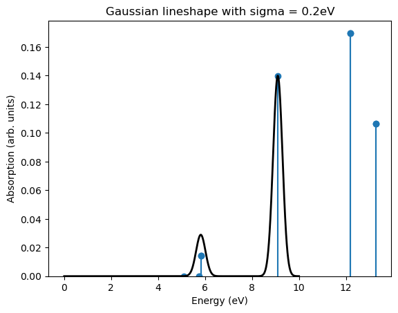
Visualize the results

Several visualisations are directly provided by pyxtp. It is for example possible to directly plot the absorption spectrum of the molecular structure assuming a Gaussian broadening of the peaks

viz = Visualization(atoms, save_figure=True)
viz.plot_absorption_gaussian()