Input files

Mapping files

Mapping relates atomistic and coarse-grained representations of the system. It is organized as follows: for each molecule type a mapping file is created. When used as a command option, these files are combined in a list separated by a semicolon, e. g. --cg protein.xml;solvent.xml.

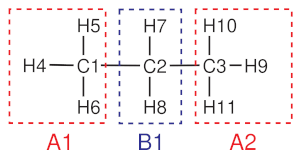
Fig. 4 Atom labeling and mapping from an all-atom to a united atom representation of a propane molecule.

Each mapping file contains a topology of the coarse-grained molecule and a list of maps. Topology specifies coarse-grained beads and bonded interactions between them. Each coarse-grained bead has a name, type, a list of atoms which belong to it, and a link to a map. A map is a set of weights \(c_{Ii}\) for an atom \(i\) belonging to the bead \(I\). It is used to calculate the position of a coarse-grained bead from the positions of atoms which belong to it. Note that \(c_{Ii}\) will be automatically re-normalized if their sum is not equal to 1, i. e. in the case of a center-of-mass mapping one can simply specify atomic masses. A complete reference for mapping file definitions can be found in Mapping file.

As an example, we will describe here a mapping file of a united atom model of a propane molecule, chemical structure of which is shown in the figure in the introduction. In this coarse-grained model, two bead types (A,B) and three beads (A1, B1, A2) are defined, as shown in the figure above. We will use the centers of mass of the beads as coarse-grained coordinates.

Extracts from the propane.xml file of the tutorial are shown below.

<cg_molecule>
  <name>ppn</name> <!-- molecule name in cg representation -->
  <ident>ppn</ident> <!-- molecule name in atomistic topology -->

  <topology> <!-- topology of one molecule -->
    <cg_beads>
      <cg_bead>  <!-- definition of a coarse-grained bead -->
        <name>A1</name>
        <type>A</type>
        <mapping>A</mapping> <!-- reference to a map -->
          <!-- atoms belonging to this bead -->
        <beads>1:ppn:C1 1:ppn:H4 1:ppn:H5 1:ppn:H6</beads>
      </cg_bead>
      <!-- more bead definitions -->
    </cg_beads>

    <cg_bonded> <!-- bonded interactions -->
      <bond>
        <name>bond</name>
        <beads>
          A1 B1
          B1 A2
        </beads>
      </bond>

      <angle>
        <name>angle</name>
        <beads>
          A1 B1 A2
        </beads>
      </angle>
    </cg_bonded>
  </topology>

  <maps>
    <map> <!-- mapping A -->
      <name>A</name>
      <weights> 12 1 1 1 </weights>
    </map>
    <!-- more mapping definitions -->
  </maps>
</cg_molecule> <!-- end of the molecule -->

An extract from the mapping file propane.xml of a propane molecule. The complete
file can be found in the csg-tutorials/propane/single_molecule tutorial

The name tag indicates the molecule name in the coarse-grained topology. The ident tag must match the name of the molecule in the atomistic representation. In the topology section all beads are defined by specifying bead name (A1, B1, A2), type, and atoms belonging to this bead in the form residue id:residue name:atom name. For each bead a map has to be specified, which is defined later in the maps section. Note that bead type and bead map can be different, which might be useful in a situation when chemically different beads (A1, B1) are assigned to the same bead type. After defining all beads, the bonded interactions of the coarse-grained molecule must be specified in the cg_bonded section. This is done by using the identifiers of the beads in the coarse-grained model. Finally, in the mapping section, the mapping coefficients are defined. This includes a weighting of the atoms in the topology section. In particular, the number of weights given should match the number of beads.

Verification of a mapping

Note that the ident tag should match the molecule name in the reference system. A common mistake occurs when beads have wrong names. In this case, the tool csg_dump can be used in order to identify the atoms which are read in from a topology file .tpr. This tool displays the atoms in the format residue id:residue name:atom name. For multicomponent systems, it might happen that molecules are not identified correctly. The workaround for this case is described in Advanced topology handling.

To compare coarse-grained and atomistic configurations one can use a standard visualization program, e. g. vmd. When comparing trajectories, one has to be careful, since vmd opens both a .gro and .trr file. The first frame is then the .gro file and the rest is taken from the .trr file. The coarse-grained trajectory contains only the frames of the trajectory. Hence, the first frame of the atomistic run has to be removed using the vmd menu.

Advanced topology handling

A topology is completely specified by a set of beads, their types, and a list of bonded interactions. VOTCA is able to read topologies in the GROMACS.tpr format. For example, one can create a coarse-grained topology based on the mapping file and atomistic GROMACS topology using csg_gmxtopol.

csg_gmxtopol --top topol.tpr --cg propane.xml --out out.top

In some cases, however, one might want to use a .pdb, H5MD or .dump file which does not contain all the required atomistic topology information. In this case, additional information can be supplied in the XMLmapping file.

A typical example is lack of a clear definition of molecules, which can be a problem for simulations with several molecules with multiple types. During coarse-graining, the molecule type is identified by a name tag as names must be clearly identified. To do this, it is possible to read a topology and then modify parts of it. The new XML topology can be used with the --tpr option, as any other topology file.

For example, if information about a molecule is not present at all, a XML topology file can be created from a .pdb file as follows

<topology base="snapshot.pdb">
  <molecules>
    <clear/>
    <define name="mCP" first="1" nbeads="52" nmols="216"/>
  </molecules>
</topology>

where <clear> clears all information that was present before.

Old versions of GROMACS did not store molecule names. In order to use this feature, a recent .tpr file containing molecule names should always be provided. For old topologies, rerun GROMACS grompp to update the old topology file.

If molecule information is already present in the parent topology but molecules are not named properly (as is the case with old GROMACS.tpr files), one can rename them using

<topology base="topol.tpr">
  <molecules>
    <rename name="PPY3" range="1:125"/>
    <rename name="Cl" range="126:250"/>
  </molecules>
</topology>

Here, the file topol.tpr is loaded first and all molecules are renamed afterwards.

If you do not have a .pdb/.gro file and you want to read trajectories from a LAMMPS .dump file or H5MD file then it is also possible to directly define the topology in a XML file. Here is an example of a XML file where the trajectory is read from a H5MD file:

<topology>
  <!-- particle group name in H5MD file -->
  <h5md_particle_group name="atoms" />
  <molecules>
    <!-- define molecule, number of beads, number of mols -->
    <molecule name="BUT" nmols="4000" nbeads="4">
      <!-- composition of molecule, bead definition -->
      <bead name="C1" type="C" mass="15.035" q="0.0" />
      <bead name="C2" type="C" mass="14.028" q="0.0" />
      <bead name="C3" type="C" mass="14.028" q="0.0" />
      <bead name="C4" type="C" mass="15.035" q="0.0" />
    </molecule>
  </molecules>
  <!-- bonded terms -->
  <bonded>
    <bond>
      <name>bond1</name>
      <beads>
        BUT:C1 BUT:C2
      </beads>
    </bond>
    <bond>
      <name>bond2</name>
      <beads>
        BUT:C2 BUT:C3
      </beads>
    </bond>
    <angle>
      <name>angle1</name>
      <beads>
        BUT:C1 BUT:C2 BUT:C3
        BUT:C2 BUT:C3 BUT:C4
      </beads>
    </angle>
    <dihedral>
      <name>dihedral1</name>
      <beads>
        BUT:C1 BUT:C2 BUT:C3 BUT:C4
      </beads>
    </dihedral>
  </bonded>
</topology>

The list of molecules is defined in section molecules where every molecule is replicated nmols times. Inside molecule, the list of bead has to be defined with the name, type, mass and charge.

The box size can be set by the tag box:

<box xx="6.0" yy="6.0" zz="6.0" />

where xx, yy, zz are the dimensions of the box.

A complete reference for a XML topology file can be found in Topology file.

Trajectories

A trajectory is a set of frames containing coordinates (velocities and forces) for the beads defined in the topology. VOTCA currently supports .trr, .xtc, .pdb, .gro and H5MD .h5 trajectory formats.

Once the mapping file is created, it is easy to convert an atomistic to a coarse-grained trajectory using csg_map.

csg_map --top topol.tpr --trj traj.trr --cg propane.xml --out cg.gro

The program csg_map also provides the option --no-map. In this case, no mapping is done and csg_map instead works as a trajectory converter. In general, mapping can be enabled and disabled in most analysis tools, e.g. in csg_stat or csg_fmatch.

Note, the topology files can have different contents as bonded interactions are not provided in all formats. In this case, mapping files can be used to define and relabel bonds.

Also note, the default settings concerning mapping varies individually between the programs. Some have a default setting that does mapping (such as csg_map, use --no-map to disable mapping) and some have mapping disabled by default (e.g. csg_stat, use --cg to enable mapping).

Setting files

<cg>
  <non-bonded> <!-- non-bonded interactions -->
    <name>A-A</name> <!-- name of the interaction -->
    <type1>A</type1> <!-- types involved in this interaction -->
    <type2>A</type2>
    <min>0</min>  <!-- dimension + grid spacing of tables-->
    <max>1.36</max>
    <step>0.01</step>
    <inverse>
      ... specific commands
    </inverse>

    ... specific section for inverse boltzmann, force matching etc.
  </non-bonded>
</cg>

Abstract of a settings.xml file. See secs. Program input, Three-body Stillinger-Weber interactions or Preparing the run for full versions.

A setting file is written in the format .xml. It consists of a general section displayed above, and a specific section depending on the program used for simulations. The setting displayed above is later extended in the sections on iterative boltzmann inversion (csg_inverse), force matching (csg_fmatch) or statistical analysis (csg_stat).

Generally, csg_stat is an analysis tool which can be used for computing radial distribution functions and analysing them. As an example, the command

csg_stat --top topol.tpr --trj traj.xtc --options settings.xml

computes the distributions of all interactions specified in settings.xml and writes all tabulated distributions as files interaction name.dist.new. A mapping file can be provided with the option --cg.

When calculating the angular distribution, an additional option <threebody> has to be added to the settings file. For example, the settings.xml file for calculating the angular distribution between three beads of type A which are all within a cutoff distance of 0.37 (nm) might look like:

<cg>
  <non-bonded> <!-- non-bonded interactions -->
    <name>A-A-A</name> <!-- name of the interaction -->
    <threebody>true</threebody> <!-- is a three-body interaction -->
    <type1>A</type1> <!-- types involved in this interaction -->
    <type2>A</type2>
    <type2>A</type2>
    <!-- dimension + grid spacing of tables-->
    <min>0</min> <!--minimum angle in radians -->
    <max>3.14</max> <!-- maximum angle in radians -->
    <step>0.02</step>
    <cut>0.37</cut>
  </non-bonded>
</cg>

In addition to distribution functions, csg_stat can also calculate the pair potential of mean force (PMF) for non-bonded pairs:

\[U_{\text{PMF}}\left(r\right)= - \int_0^r \, F_{\text{rad}}\left(r^\prime\right)\,\text{d}r^\prime.\]

The output file name is then interaction name.force.new. Here, \(F_{\text{rad}}\left(r\right)\) is the total force acting on a bead projected onto the unit distance vector connecting this pair of beads. The settings file has to contain the additional option:

<cg>
  <non-bonded> <!-- non-bonded interactions -->
    <name>A-A</name> <!-- name of the interaction -->
    <type1>A</type1> <!-- types involved in this interaction -->
    <type2>A</type2>
    <min>0</min>  <!-- dimension + grid spacing of tables-->
    <max>1.36</max>
    <step>0.01</step>
    <force>true</force>  <!-- calculate pair PMF for this interaction -->
  </non-bonded>
</cg>

Table formats

In the iterative framework distribution functions, potentials and forces are returned as tables and saved in a file. Those tables generally have the format

x y [error] flag

where x is input quantity (e.g. radius \(r\), angles \(\theta\) or \(\phi\)), y is the computed quantity (e.g. a potential) and [error] is an optional error for y. The token flag can take the values i, o or u. In the first case, i (in range) describes a value that lies within the data range, o (out of range) symbolises a value out of the data range and u stands for an undefined value.

The token flag will be important when extrapolating the table as described in Post-processing of the potential.

For historical reasons, csg_boltzmann uses a slightly different table format, it has no flag column and uses the third column as a force column when outputting a potential.