Methods
Force matching
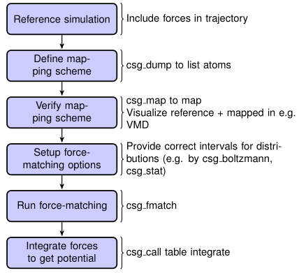
Fig. 4 Flowchart to perform force matching.
The force matching algorithm with cubic spline basis is implemented in
the utility. A list of available options can be found in the reference
section of (command –h).
Program input
csg_fmatch needs an atomistic reference run to perform coarse-graining. Therefore,
the trajectory file must contain forces (note that there is a suitable
option in the GROMACS .mdp file), otherwise csg_fmatch will not be able to
run.
In addition, a mapping scheme has to be created, which defines the
coarse-grained model (see Input files). At last, a control
file has to be created, which contains all the information for
coarse-graining the interactions and parameters for the force-matching
run. This file is specified by the tag –options in the XMLformat. An
example might look like the following
<cg>
  <!--fmatch section -->
  <fmatch>
    <!--Number of frames for block averaging -->
    <frames_per_block>6</frames_per_block>
    <!--Constrained least squares?-->
    <constrainedLS>false</constrainedLS>
  </fmatch>
  <!-- example for a non-bonded interaction entry -->
  <non-bonded>
    <!-- name of the interaction -->
    <name>CG-CG</name>
    <type1>A</type1>
    <type2>A</type2>
    <!-- fmatch specific stuff -->
    <fmatch>
      <min>0.27</min>
      <max>1.2</max>
      <step>0.02</step>
      <out_step>0.005</out_step>
    </fmatch>
  </non-bonded>
</cg>
Similarly to the case of spline fitting,
the parameters min and max have to be chosen in such a way as
to avoid empty bins within the grid. Determining min and max by
using csg_stat is recommended (see Setting files). A full description
of all available options can be found in csgapps.
Program output
csg_fmatch produces a separate .force file for each interaction, specified in
the CG-options file (--options). These files have 4 columns
containing distance, corresponding force, a table flag and the force
error, which is estimated via a block-averaging procedure. If you are
working with an angle, then the first column will contain the
corresponding angle in radians.
To get table-files for GROMACS, integrate the forces in order to get potentials and do extrapolation and potentially smoothing afterwards.
Output files are not only produced at the end of the program execution,
but also after every successful processing of each block. The user is
free to have a look at the output files and decide to stop csg_fmatch, provided
the force error is small enough.
Three-body Stillinger-Weber interactions
As described in the theory section, csg_fmatch is also able to parametrize
the angular part of three-body interactions of the Stillinger-Weber type (see subsec. Three-body Stillinger-Weber interactions).
The general procedure is the same, as shown in the two-body case
(See flowchart in Fig. Flowchart to perform force matching.).
It has to be specified in the control file that one wants to parametrize a three-body interaction. An example might look like this:
<cg>
  <!-- fmatch section -->
  <fmatch>
    <!-- Number of frames for block averaging -->
    <frames_per_block>10</frames_per_block>
    <!-- Constrained least squares?-->
    <constrainedLS>true</constrainedLS>
  </fmatch>
  <!-- example for a non-bonded interaction entry with three-body SW interactions -->
  <non-bonded>
    <!-- name of the interaction -->
    <name>CG-CG-CG</name>
    <!-- flag for three-body interactions -->
    <threebody>true</threebody>
    <!-- CG bead types (according to mapping file) -->
    <type1>A</type1>
    <type2>A</type2>
    <type3>A</type3>
    <!-- fmatch section of interaction -->
    <fmatch>
      <!-- short-range cutoff (in nm) -->
      <a>0.37</a>
      <sigma>1.0</sigma>
      <!-- switching range (steepness of exponential switching function) (in nm) -->
      <gamma>0.08</gamma>
      <!-- min for angular interaction (in rad) -->
      <min>0.7194247283</min>
      <!-- max for angular interaction (in rad) -->
      <max>3.1415927</max>
      <!-- step size for internal spline representation (in rad) -->
      <step>0.1</step>
      <!-- output step size for angular interaction (in rad) -->
      <out_step>0.0031415927</out_step>
    </fmatch>
  </non-bonded>
</cg>
As in the case of pair interactions, the parameters min and max have to be chosen in such a
way as to avoid empty bins within the grid. Determining min and max by using
csg_stat is recommended (see sec. Setting files).
For each three-body interaction as specified in the CG-options file
--options, csg_fmatch produces a separate .force file, as well as a
.pot file. Due to the functional form of the Stillinger-Weber potential,
csg_fmatch outputs the three-body force in angular direction, as well as the angular potential.
Therefore, in contrast to the two-body force (see section methods_fm_integration), the angular
three-body force does not have to be numerically integrated. The .force, as well as
the .pot file have 4 columns containing the angle in radians, the force or potential,
the error (which is estimated via a block-averaging procedure) and a table flag.
Coarse-grained simulations with three-body Stillinger-Weber interactions can be done with
LAMMPS with the MANYBODY pair_style sw/angle/table (https://docs.lammps.org/pair_sw_angle_table.html). For this, the .pot file has to be
converted into a table format according to the LAMMPS angle_style table (https://docs.lammps.org/angle_table.html).