Theoretical background

Mapping

The mapping is an operator that establishes a link between the atomistic and coarse-grained representations of the system. An atomistic system is described by specifying the values of the Cartesian coordinates and momenta

\[\begin{split}\begin{aligned} \mathbf r^n &= \{\mathbf r_1,\dots,\mathbf r_n\}, \\ \mathbf p^n &= \{\mathbf p_1,\dots,\mathbf p_n\}. \end{aligned}\end{split}\]

of the \(n\) atoms in the system. [1] On a coarse-grained level, the coordinates and momenta are specified by the positions and momenta of CG sites

\[\begin{split}\begin{aligned} \mathbf R^N = \{\mathbf R_1,\dots,\mathbf R_N\}, \\ \mathbf P^N = \{\mathbf P_1,\dots,\mathbf P_N\}. \end{aligned}\end{split}\]

Note that capitalized symbols are used for the CG sites while lower case letters are used for the atomistic system.

The mapping operator \({\mathbf c}_I\) is defined by a matrix for each bead \(I\) and links the two descriptions

\[\begin{split}\begin{aligned} {\mathbf R}_I &= \sum_{i=1}^{n}c_{Ii}\mathbf r_i, \\ {\mathbf P}_I &= M_I \dot{{\mathbf R}}_I = M_I \sum_{i=1}^{n}c_{Ii} \dot{{\mathbf r}}_i = M_I \sum_{i=1}^{n} \frac{ c_{Ii}} {m_i} {\mathbf p}_i . \end{aligned}\end{split}\]

for all \(I = 1,\dots,N\).

If an atomistic system is translated by a constant vector, the corresponding coarse-grained system is also translated by the same vector. This implies that, for all \(I\),

\[\sum_{i=1}^{n}c_{Ii}=1.\]

In some cases it is useful to define the CG mapping in such a way that certain atoms belong to several CG beads at the same time [Fritz:2009]. Following ref. [Noid:2008.1], we define two sets of atoms for each of the \(N\) CG beads. For each site \(I\), a set of involved atoms is defined as

\[{\cal I}_I=\{i|c_{Ii}\ne0\}.\]

An atom \(i\) in the atomistic model is involved in a CG site, I, if and only if this atom provides a nonzero contribution to the sum in the equation above.

A set of specific atoms is defined as

\[{\cal S}_I=\{i|c_{Ii}\ne0 \text{ and } c_{Ji}=0 \text{ for all } J \ne I\}.\]

In other words, atom \(i\) is specific to site \(I\) if and only if this atom is involved in site \(I\) and is not involved in the definition of any other site.

The CG model will generate an equilibrium distribution of momenta that is consistent with an underlying atomistic model if all the atoms are specific and if the mass of the \(I^\text{th}\) CG site is given by [Noid:2008.1]

\[M_I= \left( \sum_{i \in {\cal I}_I}\frac{c_{Ii}^2}{m_i} \right)^{-1}.\]

If all atoms are specific and the center of mass of a bead is used for mapping, then \(c_{Ii} = \frac{m_i}{M_I}\), and the condition is automatically satisfied.

Footnotes

[1]

In what follows we adopt notations of ref. [Noid:2008.1].

Boltzmann inversion

Boltzmann inversion is mostly used for bonded potentials, such as bonds, angles, and torsions [Tschoep:1998]. Boltzmann inversion is structure-based and only requires positions of atoms.

The idea of Boltzmann inversion stems from the fact that in a canonical ensemble independent degrees of freedom \(q\) obey the Boltzmann distribution, i. e.

\[P(q) = Z^{-1} \exp\left[ - \beta U(q) \right]~, \label{eq:boltzmann}\]

where is a partition function, . Once \(P(q)\) is known, one can obtain the coarse-grained potential, which in this case is a potential of mean force, by inverting the probability distribution \(P(q)\) of a variable \(q\), which is either a bond length, bond angle, or torsion angle

\[U(q) = - k_\text{B} T \ln P(q) ~. \label{eq:inv_boltzmann}\]

The normalization factor \(Z\) is not important since it would only enter the coarse-grained potential \(U(q)\) as an irrelevant additive constant.

Note that the histograms for the bonds \(H_r(r)\), angles \(H_\theta(\theta)\), and torsion angles \(H_\varphi(\varphi)\) have to be rescaled in order to obtain the volume normalized distribution functions \(P_r(r)\), \(P_\theta(\theta)\), and \(P_\varphi(\varphi)\), respectively,

\[\begin{aligned} P_r(r) = \frac{H_r(r)}{4\pi r^2}~,\; P_\theta(\theta) = \frac{H_\theta(\theta)}{\sin \theta}~,\; P_\varphi(\varphi) = H_\varphi (\varphi)~, \end{aligned}\]

where \(r\) is the bond length \(r\), \(\theta\) is the bond angle, and \(\varphi\) is the torsion angle. The bonded coarse-grained potential can then be written as a sum of distribution functions

\[\begin{split}\begin{aligned} U({r}, \theta, \varphi) &= U_r({r}) + U_{\theta}(\theta) + U_{\varphi}(\varphi)~, \\ U_q({q}) &= - k_\text{B} T \ln P_q( q ),\; q=r, \theta, \varphi~. \nonumber\end{aligned}\end{split}\]

On the technical side, the implementation of the Boltzmann inversion method requires smoothing of \(U(q)\) to provide a continuous force. Splines can be used for this purpose. Poorly and unsampled regions, that is regions with high \(U(q)\), shall be extrapolated. Since the contribution of these regions to the canonical density of states is small, the exact shape of the extrapolation is less important.

Another crucial issue is the cross-correlation of the coarse-grained degrees of freedom. Independence of the coarse-grained degrees of freedom is the main assumption that allows factorization of the probability distribution and the potential as in the above equation. Hence, one has to carefully check whether this assumption holds in practice. This can be done by performing coarse-grained simulations and comparing cross-correlations for all pairs of degrees of freedom in atomistic and coarse-grained resolution, e. g. using a two-dimensional histogram, analogous to a Ramachandran plot.  [2]

Footnotes

[2]

Checking the linear correlation coefficient does not guarantee statistical independence of variables, for example \(c(x, x^2)=0\) if \(x\) has a symmetric probability density \(P(x) = P(-x)\). This case is often encountered in systems used for coarse-graining.

Separation of bonded and non-bonded degrees of freedom

When coarse-graining polymeric systems, it is convenient to treat bonded and non-bonded interactions separately [Tschoep:1998]. In this case, sampling of the atomistic system shall be performed on a special system where non-bonded interactions are artificially removed, so that the non-bonded interactions in the reference system do not contribute to the bonded interactions of the coarse-grained model.

This can be done by employing exclusion lists using with the option --excl. This is described in detail in methods_exclusions.

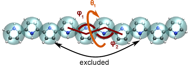
Fig. 2 Example of excluded interactions.

Force Matching

Force matching (FM) is another approach to evaluate corse-grained potentials [Ercolessi:1994,Izvekov:2005,Noid:2007]_. In contrast to the structure-based approaches, its aim is not to reproduce various distribution functions, but instead to match the multibody potential of mean force as close as possible with a given set of coarse-grained interactions.

The method works as follows. We first assume that the coarse-grained force-field (and hence the forces) depends on \(M\) parameters \(g_1,...,g_M\). These parameters can be prefactors of analytical functions, tabulated values of the interaction potentials, or coefficients of splines used to describe these potentials.

In order to determine these parameters, the reference forces on coarse-grained beads are calculated by summing up the forces on the atoms

\[{{{{\mathbf F}}}}_I^\text{ref} = \sum_{j \in {\cal S_I}} \frac{d_{Ii}}{c_{Ii}} {{{{\mathbf f}}}}_j({{{{\mathbf r}}}^n}), \label{eq:force_mapping}\]

where the sum is over all atoms of the CG site I (see Mapping). The \(d_{Ij}\) coefficients can, in principle, be chosen arbitrarily, provided that the condition :math:` sum_{i=1}^{n}d_{Ii}=1` is satisfied [Noid:2008.1]. If mapping coefficients for the forces are not provided, it is assumed that \(d_{Ij} = c_{Ij}\) (see also Input files).

By calculating the reference forces for \(L\) snapshots we can write down \(N \times L\) equations

\[{{{{\mathbf F}}}}_{Il}^\text{cg}(g_1, \dots ,g_M)={{{\mathbf F}}}_{il}^\text{ref},\; I=1,\dots,N,\; l=1,\dots,L~.\]

Here \({{{{\mathbf F}}}}_{Il}^\text{ref}\) is the force on the bead \(I\) and \({{{{\mathbf F}}}}_{Il}^\text{cg} ` is the coarse-grained representation of this force. The index :math:`l\) enumerates snapshots picked for coarse-graining. By running the simulations long enough one can always ensure that \(M < N \times L\). In this case the set of equations is overdetermined and can be solved in a least-squares manner.

\({\mathbf F}_{il}^\text{cg}\) is, in principle, a non-linear function of its parameters \(\{g_i\}\). Therefore, it is useful to represent the coarse-grained force-field in such a way that equations become linear functions of \({g_i}\). This can be done using splines to describe the functional form of the forces [Izvekov:2005]. Implementation details are discussed in ref. [Ruehle:2009.a].

Note that an adequate sampling of the system requires a large number of snapshots \(L\). Hence, the applicability of the method is often constrained by the amount of memory available. To remedy the situation, one can split the trajectory into blocks, find the coarse-grained potential for each block and then perform averaging over all blocks.

Three-body Stillinger-Weber interactions

In addition to non-bonded pair interactions, it is also possible to parametrize non-bonded three-body interactions of the Stillinger Weber type [stillinger_computer_1985]:

\[U = \sum_{I,J\neq I,K>J}f^{\left(3b\right)}\left(\theta_{IJK}\right)\,\exp{\left(\frac{\gamma_{IJ}\sigma_{IJ}}{r_{IJ}-a_{IJ}\sigma_{IJ}} + \frac{\gamma_{IK}\sigma_{IK}}{r_{IK}-a_{IK}\sigma_{IK}}\right)},\]

where \(I\) is the index of the central bead of a triplet of a CG sites, and \(J\) and \(K\) are the other two bead indices of a triplet of beads with an angular interaction term \(f^{\left(3b\right)}\left(\theta_{IJK}\right)\) and two exponential terms, \(\exp\left(\frac{\gamma\sigma}{r-a\sigma}\right)\), which guarantee a smooth switching on of the three-body forces at the cutoff distance. We do not limit ourselves to an analytic expression of \(f^{\left(3b\right)}\left(\theta_{IJK}\right)\) as in the original SW potential, but allow for a flexible angular dependence of \(f^{\left(3b\right)}\left(\theta_{IJK}\right)\). This is done by using a cubic spline representation of \(f^{\left(3b\right)}\left(\theta\right)\). Treating the two exponential terms as prefactors yields a linear dependence of the potential and thus the CG force \({\mathbf F}_{Il}^\text{cg}\) on the \(M\) spline coefficients. Therefore, the remaining parameters \(a_{IJ}\), \(a_{IK}\) (three-body short-range cutoff), \(\sigma_{IJ}\), \(\sigma_{IK}\) (additional parameter, can be set to 1), \(\gamma_{IJ}\), and \(\gamma_{IK}\) (steepness of switching), have to be set before solving the set of linear equations. For a more detailed description, we refer to ref. [scherer_understanding_2018].